Kubeflow Pipelines v2 実践ガイド — KFP SDKでMLパイプラインを構築する

• はじめに
• KFP v2のインストールと基本概念
  • インストール
  • 基本概念
• コンポーネントの定義
  • 軽量Pythonコンポーネント
  • カスタムDockerイメージコンポーネント
• パイプラインの作成
  • 基本パイプライン
  • パイプラインのコンパイルと実行
  • 定期実行（Recurring Run）
• 高度なパターン
  • 並列実行（ParallelFor）
  • キャッシング
  • ボリュームマウント
• CI/CD統合
  • GitHub Actions + KFP
• コンパイルすると何が出てくるのか
• 実行を送信してランを読む方法
• 最初から最後まで一度回してみる
• コンポーネントは想像以上に孤立している
• 失敗したランを読む順番
• キャッシングはデフォルトで有効になっている
• 制御フローとプラットフォーム機能は名前が変わった
• KFPを使わないほうがいい場合
• まとめ
• 参考資料
• クイズ

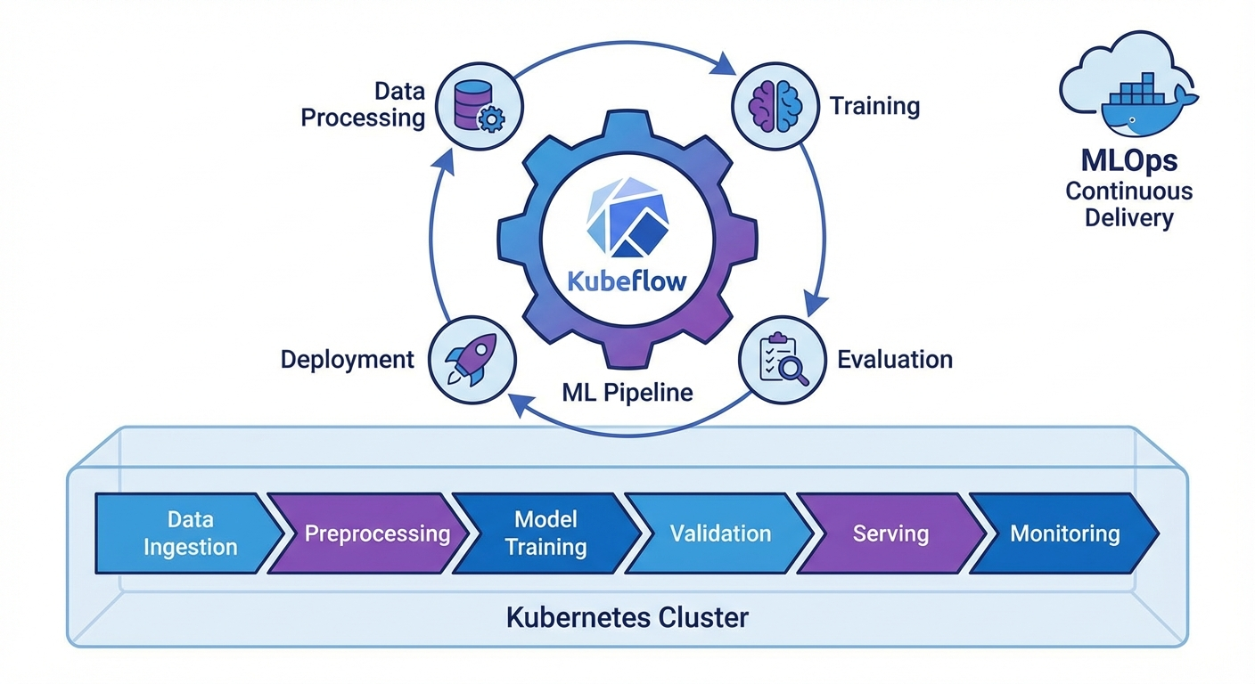
はじめに

MLモデルを実験からプロダクションに移行する過程で、再現性、自動化、バージョン管理は必須です。Kubeflow Pipelines（KFP）v2はKubernetes上でMLワークフローを定義・実行するフレームワークで、Pythonデコレータだけでパイプラインを構成できます。

本記事では、KFP v2 SDKの主要機能と実践的なパイプライン構築を解説します。

KFP v2のインストールと基本概念

インストール

pip install kfp==2.7.0

# Kubeflow Pipelinesバックエンドのインストール（Kubernetes）
kubectl apply -k "github.com/kubeflow/pipelines/manifests/kustomize/env/platform-agnostic?ref=2.2.0"

# ポートフォワーディング
kubectl port-forward svc/ml-pipeline-ui -n kubeflow 8080:80

基本概念

# 1. Component: パイプラインの作業単位（Python関数）
# 2. Pipeline: ComponentのDAG（有向非巡回グラフ）
# 3. Artifact: 入出力データ（Dataset, Model, Metricsなど）
# 4. Run: パイプラインの1回の実行
# 5. Experiment: Runの論理的なグループ

コンポーネントの定義

軽量Pythonコンポーネント

from kfp import dsl
from kfp.dsl import (
    Dataset, Input, Output, Model, Metrics,
    ClassificationMetrics, component
)


@dsl.component(
    base_image="python:3.11-slim",
    packages_to_install=["pandas==2.1.4", "scikit-learn==1.4.0"]
)
def load_data(
    dataset_url: str,
    output_dataset: Output[Dataset]
):
    """データ読み込みコンポーネント"""
    import pandas as pd

    df = pd.read_csv(dataset_url)
    print(f"Loaded {len(df)} rows")

    # 出力アーティファクトに保存
    df.to_csv(output_dataset.path, index=False)
    output_dataset.metadata["num_rows"] = len(df)
    output_dataset.metadata["num_columns"] = len(df.columns)


@dsl.component(
    base_image="python:3.11-slim",
    packages_to_install=["pandas==2.1.4", "scikit-learn==1.4.0"]
)
def preprocess_data(
    input_dataset: Input[Dataset],
    train_dataset: Output[Dataset],
    test_dataset: Output[Dataset],
    test_size: float = 0.2
):
    """データの前処理と分割"""
    import pandas as pd
    from sklearn.model_selection import train_test_split

    df = pd.read_csv(input_dataset.path)

    # 前処理
    df = df.dropna()
    df = df.drop_duplicates()

    # 分割
    train_df, test_df = train_test_split(df, test_size=test_size, random_state=42)

    train_df.to_csv(train_dataset.path, index=False)
    test_df.to_csv(test_dataset.path, index=False)

    train_dataset.metadata["num_rows"] = len(train_df)
    test_dataset.metadata["num_rows"] = len(test_df)


@dsl.component(
    base_image="python:3.11-slim",
    packages_to_install=[
        "pandas==2.1.4", "scikit-learn==1.4.0",
        "joblib==1.3.2", "xgboost==2.0.3"
    ]
)
def train_model(
    train_dataset: Input[Dataset],
    model_output: Output[Model],
    metrics_output: Output[Metrics],
    n_estimators: int = 100,
    max_depth: int = 6,
    learning_rate: float = 0.1
):
    """モデル学習"""
    import pandas as pd
    import joblib
    from xgboost import XGBClassifier
    from sklearn.model_selection import cross_val_score

    df = pd.read_csv(train_dataset.path)
    X = df.drop("target", axis=1)
    y = df["target"]

    # 学習
    model = XGBClassifier(
        n_estimators=n_estimators,
        max_depth=max_depth,
        learning_rate=learning_rate,
        random_state=42
    )
    model.fit(X, y)

    # 交差検証
    cv_scores = cross_val_score(model, X, y, cv=5, scoring="accuracy")

    # モデル保存
    joblib.dump(model, model_output.path)
    model_output.metadata["framework"] = "xgboost"
    model_output.metadata["n_estimators"] = n_estimators

    # メトリクス記録
    metrics_output.log_metric("cv_accuracy_mean", float(cv_scores.mean()))
    metrics_output.log_metric("cv_accuracy_std", float(cv_scores.std()))
    metrics_output.log_metric("n_estimators", n_estimators)


@dsl.component(
    base_image="python:3.11-slim",
    packages_to_install=[
        "pandas==2.1.4", "scikit-learn==1.4.0",
        "joblib==1.3.2", "xgboost==2.0.3"
    ]
)
def evaluate_model(
    test_dataset: Input[Dataset],
    model_input: Input[Model],
    metrics_output: Output[ClassificationMetrics],
    eval_metrics: Output[Metrics]
) -> float:
    """モデル評価"""
    import pandas as pd
    import joblib
    from sklearn.metrics import accuracy_score, classification_report

    df = pd.read_csv(test_dataset.path)
    X = df.drop("target", axis=1)
    y = df["target"]

    model = joblib.load(model_input.path)
    y_pred = model.predict(X)
    y_prob = model.predict_proba(X)

    accuracy = accuracy_score(y, y_pred)

    # 分類メトリクス（混同行列の可視化）
    metrics_output.log_confusion_matrix(
        categories=["Class 0", "Class 1"],
        matrix=[[int(sum((y == 0) & (y_pred == 0))), int(sum((y == 0) & (y_pred == 1)))],
                [int(sum((y == 1) & (y_pred == 0))), int(sum((y == 1) & (y_pred == 1)))]]
    )

    eval_metrics.log_metric("test_accuracy", accuracy)

    return accuracy

カスタムDockerイメージコンポーネント

@dsl.component(
    base_image="pytorch/pytorch:2.1.0-cuda12.1-cudnn8-runtime",
    packages_to_install=["transformers==4.37.0", "datasets==2.16.0"]
)
def finetune_llm(
    model_name: str,
    train_dataset: Input[Dataset],
    output_model: Output[Model],
    epochs: int = 3,
    batch_size: int = 8
):
    """LLMファインチューニング（GPU使用）"""
    from transformers import AutoModelForSequenceClassification, Trainer
    # ... 学習コード
    pass

パイプラインの作成

基本パイプライン

@dsl.pipeline(
    name="ML Training Pipeline",
    description="データ読み込み → 前処理 → 学習 → 評価パイプライン"
)
def ml_training_pipeline(
    dataset_url: str = "https://example.com/data.csv",
    test_size: float = 0.2,
    n_estimators: int = 100,
    max_depth: int = 6,
    learning_rate: float = 0.1,
    accuracy_threshold: float = 0.85
):
    # Step 1: データ読み込み
    load_task = load_data(dataset_url=dataset_url)

    # Step 2: 前処理（load_task完了後に実行）
    preprocess_task = preprocess_data(
        input_dataset=load_task.outputs["output_dataset"],
        test_size=test_size
    )

    # Step 3: モデル学習
    train_task = train_model(
        train_dataset=preprocess_task.outputs["train_dataset"],
        n_estimators=n_estimators,
        max_depth=max_depth,
        learning_rate=learning_rate
    )
    # リソース制限の設定
    train_task.set_cpu_limit("4")
    train_task.set_memory_limit("8Gi")

    # Step 4: 評価
    eval_task = evaluate_model(
        test_dataset=preprocess_task.outputs["test_dataset"],
        model_input=train_task.outputs["model_output"]
    )

    # Step 5: 条件付きデプロイ
    with dsl.If(eval_task.output >= accuracy_threshold):
        deploy_task = deploy_model(
            model_input=train_task.outputs["model_output"],
            accuracy=eval_task.output
        )


@dsl.component(base_image="python:3.11-slim")
def deploy_model(
    model_input: Input[Model],
    accuracy: float
):
    """モデルデプロイ（条件充足時）"""
    print(f"Deploying model with accuracy: {accuracy:.4f}")
    print(f"Model path: {model_input.path}")
    # 実際のデプロイロジック（K8s Serving、BentoMLなど）

パイプラインのコンパイルと実行

from kfp import compiler
from kfp.client import Client

# 1. YAMLにコンパイル
compiler.Compiler().compile(
    pipeline_func=ml_training_pipeline,
    package_path="ml_pipeline.yaml"
)

# 2. KFPサーバーに送信
client = Client(host="http://localhost:8080")

# Experimentの作成
experiment = client.create_experiment(name="ml-experiments")

# Runの実行
run = client.create_run_from_pipeline_func(
    ml_training_pipeline,
    experiment_name="ml-experiments",
    run_name="training-run-001",
    arguments={
        "dataset_url": "gs://my-bucket/data.csv",
        "n_estimators": 200,
        "max_depth": 8,
        "accuracy_threshold": 0.90
    }
)

print(f"Run ID: {run.run_id}")
print(f"Run URL: http://localhost:8080/#/runs/details/{run.run_id}")

定期実行（Recurring Run）

# 毎日午前2時に実行
client.create_recurring_run(
    experiment_id=experiment.experiment_id,
    job_name="daily-retraining",
    pipeline_func=ml_training_pipeline,
    cron_expression="0 2 * * *",
    max_concurrency=1,
    arguments={
        "dataset_url": "gs://my-bucket/latest-data.csv",
        "accuracy_threshold": 0.85
    }
)

高度なパターン

並列実行（ParallelFor）

@dsl.pipeline(name="Hyperparameter Search")
def hp_search_pipeline():
    # ハイパーパラメータの組み合わせを定義
    hp_configs = [
        {"n_estimators": 100, "max_depth": 4, "lr": 0.1},
        {"n_estimators": 200, "max_depth": 6, "lr": 0.05},
        {"n_estimators": 300, "max_depth": 8, "lr": 0.01},
    ]

    # 並列学習
    with dsl.ParallelFor(hp_configs) as config:
        train_task = train_model(
            train_dataset=load_task.outputs["output_dataset"],
            n_estimators=config.n_estimators,
            max_depth=config.max_depth,
            learning_rate=config.lr
        )

キャッシング

# コンポーネントレベルでキャッシュを無効化
load_task = load_data(dataset_url=dataset_url)
load_task.set_caching_options(False)  # 常に再実行

# パイプラインレベルでキャッシュを設定
run = client.create_run_from_pipeline_func(
    ml_training_pipeline,
    enable_caching=True  # 同一入力の場合はキャッシュを使用
)

ボリュームマウント

@dsl.component(base_image="python:3.11-slim")
def process_large_data(output_data: Output[Dataset]):
    """大容量データの処理"""
    pass

# PVCマウント
process_task = process_large_data()
process_task.add_pvolumes({
    "/mnt/data": dsl.PipelineVolume(pvc="data-pvc")
})

CI/CD統合

GitHub Actions + KFP

# .github/workflows/ml-pipeline.yml
name: ML Pipeline CI/CD

on:
  push:
    branches: [main]
    paths:
      - 'pipelines/**'
      - 'components/**'

jobs:
  deploy-pipeline:
    runs-on: ubuntu-latest
    steps:
      - uses: actions/checkout@v4

      - name: Set up Python
        uses: actions/setup-python@v5
        with:
          python-version: '3.11'

      - name: Install dependencies
        run: pip install kfp==2.7.0

      - name: Compile pipeline
        run: python pipelines/compile.py

      - name: Upload and run pipeline
        env:
          KFP_HOST: ${{ secrets.KFP_HOST }}
        run: |
          python -c "
          from kfp.client import Client
          client = Client(host='$KFP_HOST')
          client.upload_pipeline(
            pipeline_package_path='ml_pipeline.yaml',
            pipeline_name='ml-training-v2',
            description='Automated ML training pipeline'
          )
          "

コンパイルすると何が出てくるのか

まずバージョンです。この節以降のAPIはkfp SDK 2.17.0を基準にしており、kfp-kubernetes 2.17.0とkfp-server-api 2.17.0を一緒に使います。Python 3.9以上が必要で、上のインストールブロックの2.7.0とは異なります。見つけた例がそのまま動かないなら、十中八九SDKのバージョン差です。

APIリファレンスはCompilerを「KFP SDK DSLで記述したパイプラインをYAMLパイプライン定義にコンパイルする」と説明し、package_pathを「出力YAMLファイルのパス」と明記しています。v2のコンパイル成果物は、常にYAMLファイル1つです。

from kfp import compiler

compiler.Compiler().compile(
    pipeline_func=ml_training_pipeline,
    package_path="ml_pipeline.yaml",  # ドキュメントの表現どおり「出力YAMLファイルのパス」
    pipeline_name="ml-training",
    pipeline_display_name="ML Training Pipeline",
    pipeline_parameters={"n_estimators": 200},
    type_check=True,
)
# 残りの引数: kubernetes_manifest_options, kubernetes_manifest_format
# 注意: kfp_package_path は compile() ではなく @dsl.component の引数だ

コンパイルはクラスタにもバックエンドにも触れません。だからこそ、CIで最初に回すべき検査です。タスクの接続を間違えたり型が合わなかったりすれば、ここで引っかかります。CIのステップを1行で済ませたいならCLIが楽です。

kfp dsl compile --py my_pipeline.py --output my_pipeline.yaml

kfp_package_pathはコンパイルのオプションのように見えるので、ここで迷う人が多いです。kubernetes_manifest_optionsのように名前だけでは用途がはっきりしない引数は、正確なAPIを使っているバージョンのドキュメントで確認してください。

実行を送信してランを読む方法

上げる経路は2つあります。create_run_from_pipeline_funcはパイプライン関数を受け取って内部でコンパイルまで行い、create_run_from_pipeline_packageは作っておいたYAMLを受け取ります。引数のセットは同じです。実務では後者を勧めます。CIで作ったYAML1つを、ステージングにもプロダクションにもそのまま上げられます。

from kfp.client import Client

client = Client(host="http://localhost:8080", namespace="kubeflow")
experiment = client.create_experiment(name="ml-experiments")

# 2つの関数に共通する引数: arguments, run_name, experiment_name, namespace,
#   pipeline_root, enable_caching, cache_key, service_account, experiment_id
run = client.create_run_from_pipeline_package(
    pipeline_file="ml_pipeline.yaml",
    arguments={"n_estimators": 200, "accuracy_threshold": 0.90},
    run_name="training-run-001",
    experiment_id=experiment.experiment_id,
    enable_caching=True,
)

# CI ではここでブロックしないと終了コードに成否が伝わらない
client.wait_for_run_completion(run.run_id, timeout=3600, sleep_duration=5)

# カタログへの登録とバージョン上げ
client.upload_pipeline("ml_pipeline.yaml", pipeline_name="ml-training-v2")
client.upload_pipeline_version("ml_pipeline.yaml", "v3", pipeline_name="ml-training-v2")

# 定期実行は関数ではなくパッケージか登録済みパイプラインを指す
client.create_recurring_run(
    experiment_id=experiment.experiment_id,
    job_name="daily-retraining",
    pipeline_package_path="ml_pipeline.yaml",  # または pipeline_id / version_id
    cron_expression="0 2 * * *",
    max_concurrency=1,
    no_catchup=True,      # 止まってから復帰しても、たまったスケジュールをまとめて回さない
    params={"accuracy_threshold": 0.85},
)

Clientのデフォルトのネームスペースはkubeflowで、list_runsはデフォルトのpage_sizeが10なので10件しか返ってきません。

定期実行には落とし穴があります。上のほうの例はcreate_recurring_runにpipeline_funcを渡していますが、確認したシグネチャにそんな引数はありません。関数ではなく、コンパイル済みのパッケージか登録済みパイプラインのIDを指す必要があります。

ランが始まると、グラフのノード1つがタスク1つで、タスク1つがPod1つです。ノードをクリックすると、ログと入出力アーティファクト、キャッシュヒットの有無が見えます。Pod名の規則とラベルはデプロイ方式によって違うので、使っているデプロイのドキュメントで確認してください。

最初から最後まで一度回してみる

上のほうの例は外部のCSVとXGBoostが必要で、そのまま回すのは難しいです。ここではコピーしてすぐ送信できる最小のパイプラインを作ってみます。目的は、コンパイルから送信を経てアーティファクトがUIに出るまでの経路を一度通すことです。

from typing import NamedTuple

from kfp import compiler, dsl
from kfp.client import Client


@dsl.component(base_image="python:3.11")
def make_split(n_rows: int, ratio: float) -> NamedTuple('outputs', train=int, test=int):
    from typing import NamedTuple

    outputs = NamedTuple('outputs', train=int, test=int)
    n_test = int(n_rows * ratio)
    return outputs(n_rows - n_test, n_test)


@dsl.component(base_image="python:3.11", packages_to_install=["scikit-learn==1.4.0"])
def fit_and_score(
    train_rows: int,
    model: dsl.Output[dsl.Model],
    metrics: dsl.Output[dsl.Metrics],
):
    import json

    from sklearn.dummy import DummyClassifier

    X = [[0], [1]] * train_rows
    y = [0, 1] * train_rows

    clf = DummyClassifier(strategy="most_frequent")
    clf.fit(X, y)
    accuracy = float(clf.score(X, y))

    with open(model.path, "w") as f:
        json.dump({"strategy": "most_frequent"}, f)
    model.metadata["framework"] = "sklearn"
    metrics.log_metric("accuracy", accuracy)


@dsl.pipeline(name="smoke-pipeline", description="compile to submit smoke test")
def smoke_pipeline(n_rows: int = 1000, ratio: float = 0.2):
    split = make_split(n_rows=n_rows, ratio=ratio)

    fit = fit_and_score(train_rows=split.outputs["train"])
    fit.set_memory_request("512Mi")
    fit.set_memory_limit("1Gi")
    fit.set_retry(num_retries=2)


compiler.Compiler().compile(smoke_pipeline, package_path="smoke_pipeline.yaml")

client = Client(host="http://localhost:8080")
run = client.create_run_from_pipeline_package(
    "smoke_pipeline.yaml",
    arguments={"n_rows": 1000},
    run_name="smoke-001",
    experiment_name="smoke",
)
print(run.run_id)
client.wait_for_run_completion(run.run_id, timeout=900)

# パラメータのマッピング: str -> string, int/float -> number, bool -> boolean,
#                        list/dict -> object
# アーティファクトの型: dsl.Artifact(system.Artifact), Dataset, Model, Metrics,
#   ClassificationMetrics, SlicedClassificationMetrics, HTML, Markdown
#   共通の属性 .name .uri .path .metadata / Model には .framework が追加される
# Metrics.log_metric(metric, value)
# ClassificationMetrics.log_roc_data_point(fpr, tpr, threshold), log_roc_curve(),
#   set_confusion_matrix_categories(), log_confusion_matrix_row(),
#   log_confusion_matrix_cell(), log_confusion_matrix(categories, matrix)
# dsl.InputPath / dsl.OutputPath は主に Container Components 用で、
#   Python Components は戻り値の型アノテーションで同じことをする

回すとだいたいこういう形になります。文字列とUIの配置はバックエンドのバージョンごとに違うので、各項目があるかどうかだけ見れば十分です。

1) コンパイル成果物
   smoke_pipeline.yaml          <- ファイル1つだけだ

2) 送信直後の標準出力
   ランIDがUUID1行で表示される

3) UIのラン詳細画面のグラフ
   make_split       Succeeded
   fit_and_score    Succeeded
     Metrics   タブ : accuracy = 0.5
     Artifacts タブ : model (system.Model), metadata.framework = sklearn

4) 同じ引数でもう一度送信すると
   make_split       Succeeded  (キャッシュヒット表示)
   fit_and_score    Succeeded  (キャッシュヒット表示)
   -> 実行時間が数秒に縮む

新しいクラスタを検収するときは、最初の実行が成功するか、2回目が速くなるか、この2つを見るだけでバックエンドとアーティファクトストレージがつながっているサインになります。

出力が複数あるコンポーネントはNamedTupleで宣言し、次のタスクでtask.outputs['<output-key>']から取り出します。NamedTupleを関数の中で定義し直す不格好なコードはミスではなく必須で、理由は次の節で説明します。

小さい値はパラメータとしてシリアライズされ、モデルやデータセットのような大きいものはアーティファクトになります。型ごとのマッピングとメソッド名は、上のコード末尾のコメントにあります。1つだけ挙げると、ROCの点を打つメソッドはlog_roc_data_pointで、例でときどき見かけるlog_roc_readingという名前は存在しません。

コンポーネントは想像以上に孤立している

いちばん多く踏む落とし穴です。ドキュメントはPythonコンポーネントに2つの制約を明示しています。関数の入力と出力には有効なKFPの型アノテーションが必要で、関数はその本体の外で定義されたどんなシンボルも参照できません。

本命は2つ目です。デコレータは関数のソースを切り出してコンテナの中で単独で実行するので、モジュール上部のimportもファイルのどこかにある定数も、コンテナの中には存在しません。

# 動作しない - 本体の外のシンボルを参照している
import pandas as pd

TARGET_COLUMN = "label"


@dsl.component(base_image="python:3.11")
def bad_component(data: dsl.Input[dsl.Dataset]) -> int:
    df = pd.read_csv(data.path)                # NameError: name 'pd' is not defined
    return int(df[TARGET_COLUMN].nunique())    # NameError: name 'TARGET_COLUMN' ...


# 動作する - すべてのシンボルが本体の中にある
@dsl.component(base_image="python:3.11", packages_to_install=["pandas==2.1.4"])
def good_component(data: dsl.Input[dsl.Dataset], target_column: str = "label") -> int:
    import pandas as pd

    df = pd.read_csv(data.path)
    return int(df[target_column].nunique())

厄介なのは、コンパイルが通ってしまうところです。YAMLが作られ、ランも始まったあとに、クラスタでNameErrorで落ちます。レビューのルールは1つで足ります。コンポーネント関数の1行目はimportであるべきで、シグネチャにない名前が本体にあれば差し戻します。

packages_to_installにも代償があります。ドキュメントは、このリストがタスクの実行のたびにインストールされると説明しています。100回回せばpip installも100回走ります。代替は、依存をビルド時にイメージへ焼き込むContainerized Python Componentsです。

# イメージだけ作ってプッシュしない (ローカル確認用)
kfp component build src/ --component-filepattern my_component.py --no-push-image

# レジストリまで上げる (CIで使う形)
kfp component build src/ --component-filepattern my_component.py --push-image

base_imageのデフォルトは、Containerized Python Componentsのドキュメント基準でpython:3.11です。ただしLightweight Python Componentsのページにはまだpython:3.7と書かれていて2つのページが食い違っているので、常に明示してください。閉域網ではpip_index_urls、pip_trusted_hosts、install_kfp_package、use_venvが一緒に必要になります。

失敗したランを読む順番

ランが赤くなったら、UIを眺めずに順番に進みます。失敗したノードを見つけ、ログの最後の30行だけを読み、Pythonの例外なのかPodが立ち上がらなかったのかを切り分けます。

• NameErrorまたはModuleNotFoundError — 隔離ルールの違反か、パッケージの不足です。コンパイルが通ったことに意味はありません。
• 次のタスクが入力を見つけられない — .uriに直接書いた場合です。ドキュメントの表現では、.uriはアーティファクトがストレージ上に実際に存在する場所で、.pathは便利なローカルファイルシステムアクセスを提供します。コードは.pathに書きます。
• PodがPendingから動かない — requestはスケジューリングの基準、limitは上限です。requestだけ大きく取ると永遠にPendingで、Kubernetesのイベントに出ます。
• GPUタスクがGPUなしで立ち上がる — set_accelerator_typeとset_accelerator_limitを両方かけたか見ます。set_gpu_limitは現在のリファレンスにありません。
• イメージを取得できない — KFPではなくKubernetes一般の動作なので、クラスタ側のドキュメントを見ます。
• すぐ終わる — 失敗ではなくキャッシュヒットです。

リトライはset_retry(num_retries, backoff_duration=None)、前段が失敗しても進めたい後始末はignore_upstream_failure()です。全体の成否に反応するにはdsl.ExitHandlerとdsl.PipelineTaskFinalStatusの組み合わせで、stateはSUCCEEDED、FAILED、CANCELLEDのいずれかです。

@dsl.component(base_image="python:3.11")
def notify(status: dsl.PipelineTaskFinalStatus):
    print("state:", status.state)
    if status.state == "FAILED":
        print("pipeline failed - send alert here")


@dsl.pipeline(name="pipeline-with-exit-handler")
def pipeline_with_exit_handler(n_rows: int = 1000):
    with dsl.ExitHandler(exit_task=notify()):
        split = make_split(n_rows=n_rows, ratio=0.2)

        fit = fit_and_score(train_rows=split.outputs["train"])
        fit.set_retry(num_retries=2)

夜間の再学習が静かに失敗する状況は、これで防ぎます。backoff_durationが受け取る値の形式は確認できなかったので、正確なAPIは使っているバージョンのドキュメントで確認してください。

キャッシングはデフォルトで有効になっている

ドキュメントは、すべてのコンポーネントに対してキャッシングがデフォルトで有効だと明記しています。有効にするのではなく、すでに有効で、必要なときに切るものです。

設定は3つの層です。タスク単位はset_caching_options(False)、ラン単位はenable_cachingで、ラン単位がタスク単位を上書きします。コンポーネントで切ったのにヒットするなら、ランの引数を見てください。

# 1) タスク単位 - このタスクだけ常に新しく実行する
load_task = load_data(dataset_url=dataset_url)
load_task.set_caching_options(False)

# 2) ラン単位 - タスク単位の設定を上書きする
run = client.create_run_from_pipeline_func(
    ml_training_pipeline,
    arguments={"dataset_url": "gs://my-bucket/data.csv"},
    enable_caching=False,
)

3つ目は全体です。コンパイルフラグか環境変数でデフォルト値そのものを切れますが、環境変数はコンポーネントをimportする前に設定しないと効きません。

# コンパイルフラグでデフォルト値を切る
kfp dsl compile --py my_pipeline.py --output my_pipeline.yaml \
  --disable-execution-caching-by-default

# または環境変数で (コンポーネントを import する前に設定する必要がある)
export KFP_DISABLE_EXECUTION_CACHING_BY_DEFAULT=true
python my_pipeline.py

キャッシュがヒットすると、UIに緑の雲と矢印のアイコンが付きます。

ここからはドキュメントではなく推測です。キャッシュキーの構成要素はドキュメント化されていないので断定できません。ただ、コンポーネントと入力がそのままなら以前の出力が返ってくるという観察から見ると、驚く状況はたいてい、変わったものがキャッシュキーの外にある場合です。外部バケットのデータが静かに更新されたり、latestのような浮動タグのイメージが差し替わったりした場合が代表的です。疑わしければ、そのタスクだけキャッシングを切って比べてください。

制御フローとプラットフォーム機能は名前が変わった

古いコードを移すとき最初に確認する名前はdsl.Conditionです。ドキュメントは、これが機能的に同等なdsl.Ifに置き換えられて非推奨になったと明記しています。上のパイプラインはすでにdsl.Ifを使っていますが、社内リポジトリのv2初期コードには残っているはずです。

分岐はdsl.If、dsl.Elif、dsl.Elseで完結し、分岐ごとに違うタスクの出力を1つで受けるときはdsl.OneOfです。ここにはdsl.Elseの分岐が必ず必要です。並列実行で見落としやすい引数は、dsl.ParallelFor(items, name=None, parallelism=None)のparallelismです。そのまま展開すると組み合わせの数だけPodが一度に立ち上がり、クラスタが小さいと全部Pendingにかかります。ファンアウトの結果をまとめるときはdsl.Collectedです。

@dsl.pipeline(name="control-flow-example")
def control_flow_example(threshold: float = 0.85):
    # train_with_epochs, max_accuracy, promote_model, stage_model,
    # report_failure はそれぞれ自分で定義したコンポーネントだと仮定する

    # parallelism で同時に立ち上がる Pod の数を制限する
    with dsl.ParallelFor(items=[1, 5, 10, 25], parallelism=2) as epochs:
        train_task = train_with_epochs(epochs=epochs)

    # ファンアウトした結果を1つにまとめる
    best = max_accuracy(models=dsl.Collected(train_task.outputs["model"]))

    with dsl.If(best.output >= threshold):
        promote_model(score=best.output)
    with dsl.Elif(best.output >= 0.70):
        stage_model(score=best.output)
    with dsl.Else():
        report_failure(score=best.output)

# PipelineTask の確認されたメソッド (すべてチェーンできる)
#   set_cpu_request, set_cpu_limit, set_memory_request, set_memory_limit,
#   set_accelerator_type, set_accelerator_limit, set_caching_options,
#   set_retry, set_env_variable, ignore_upstream_failure, after
#   set_gpu_limit は現在の API リファレンスにない

ボリュームは別パッケージです。上のボリュームマウント例のadd_pvolumesとdsl.PipelineVolumeはKFP v1系の表記で、v2で確認された経路はpip install kfp[kubernetes]でインストールするkfp-kubernetesです。

from kfp import dsl, kubernetes


@dsl.pipeline(name="pvc-example")
def pvc_example():
    pvc1 = kubernetes.CreatePVC(
        pvc_name_suffix='-my-pvc',
        access_modes=['ReadWriteMany'],
        size='5Gi',
        storage_class_name='standard',
    )

    task1 = producer()
    kubernetes.mount_pvc(task1, pvc_name=pvc1.outputs['name'], mount_path='/data')

    task2 = consumer().after(task1)
    kubernetes.mount_pvc(task2, pvc_name=pvc1.outputs['name'], mount_path='/data')

    # 後片付けまでパイプラインの中で終わらせる
    kubernetes.DeletePVC(pvc_name=pvc1.outputs['name']).after(task2)


# 同じパッケージで確認された他の機能
#   use_secret_as_env, use_secret_as_volume, use_config_map_as_env,
#   use_config_map_as_volume, add_ephemeral_volume, add_pod_label,
#   add_pod_annotation, use_field_path_as_env, set_timeout,
#   set_image_pull_policy, set_security_context, set_image_pull_secrets

GPUクラスタでよく必要になるノード選択やtaintの回避のような機能の関数名は確認できなかったので、正確なAPIは使っているバージョンのドキュメントで確認してください。

KFPを使わないほうがいい場合

KFPは軽い道具ではありません。パイプラインを1つ回すのに、Kubernetesクラスタ、KFPバックエンド、オブジェクトストレージがすべて生きている必要があります。その対価として得られる再現性と系譜追跡が要らない仕事に付けると、コストだけが残ります。

• Pythonスクリプト1つで終わる仕事 — コンポーネントに分けた瞬間、段階の間のデータはシリアライズされてストレージを往復します。数秒の作業ではオーバーヘッドのほうが作業より大きくなります。
• 決まった時刻に同じことを回すだけの場合 — 系譜を見ることがないなら、cronやKubernetesのCronJobで十分です。
• Kubernetesを読める人がいない場合 — KFPの失敗の大半はKubernetesから来ます。クラスタを読める人がいないと、デバッグが占いになります。
• チームがすでに別のオーケストレータに定着している場合 — 学習ジョブを既存のツールから呼ぶほうがだいたい安上がりです。
• まだ探索段階 — 毎回イメージを作ったりpip installを待ったりした瞬間、反復の速度が崩れます。

逆にKFPが価値を出す地点は、狭くて明確です。複数人が同じ学習を回しているのに結果が違うとき、3か月前のモデルがどんなデータで作られたのかを遡る必要があるときです。

まとめ

Kubeflow Pipelines v2の要点整理：

1. @dsl.component: Python関数をコンテナ化されたコンポーネントに変換
2. @dsl.pipeline: コンポーネントをDAGとして接続
3. Artifactシステム: Dataset、Model、Metricsタイプで入出力を管理
4. 条件/繰り返し: dsl.If、dsl.ParallelForで動的パイプラインを構築
5. キャッシング: 同一入力時の再実行を防止してコストを削減

実際に時間を食うのはこの5つではなく、隔離のルールとデフォルトで有効なキャッシングです。

参考資料

同じ内容がページごとに違って書かれていることもありますが、そういうときはreadthedocs側のほうが実際のシグネチャに近いです。

• dsl - 2026-08-16確認。
• compiler - 2026-08-16確認。
• client - 2026-08-16確認。
• Containerized Python Components - 2026-08-16確認。
• Artifacts - 2026-08-16確認。
• Control flow - 2026-08-16確認。
• Caching - 2026-08-16確認。
• Platform-specific features - 2026-08-16確認。

クイズ